Riddler Classic: How Low Can You Roll?

What’s the average score of the game?

In this week’s FiveThirtyEight Riddler Classic we are asked to calculate the average of series of scores, based on rolls of classic D&D style 10-sided die. The twist is that your score is the value of the die divided by 10, and you keep rolling the die over and over until you roll a zero. Each time you roll, if the digit shown by the die is less than or equal to the last digit of your score, then that roll becomes the new last digit of your score. Otherwise you just go ahead and roll again until you roll a zero.

I simulated one game in R as show below. I generate 150 digits between 0-9 (just to be safe) and keep them until hitting the first zero. Then I check every digit and eliminate it if it’s greater than the prior digit. Last step is to divide each digit by the appropriate power of 10 and sum them.

roll <- function() {
    draws <- sample(0:9, 150, replace = T)
    if (draws[1]==0) return(0)
    draws <- draws[1:min(which(draws==0))]
    lastgood <- draws[1]

for (i in 2:length(draws)){
  
  if (draws[i]==0) break
  if (draws[i] > lastgood) {draws[i] <- NA}
  else lastgood <- draws[i]
                          }
draws <- draws[!is.na(draws)]

return(sum(draws/(10^seq_along(draws))))
}

roll()

## [1] 0.2

Next, I create a function to generate n such digits, as well as a function to create a table with them and compute the rolling average:

roll_n <- function(n){
  output <- numeric(n)
  for (i in seq_len(n)) output[i] <- roll()
  return(output)
}
roll_n(3)

## [1] 0.000000 0.210000 0.621111

mc_table <- function(n, cumavg=T){
  
  output <- matrix(data=NA, nrow=n, ncol=3)
  output <- as.data.frame(output)
  output[ ,1] <- 1:n
  output[ ,2] <- roll_n(n)
  if (cumavg) output[, 3] <- cumsum(output[,2]) / output[,1]
  colnames(output) <- c("n", "roll", "cumavg")
  return(output)
}

Let’s run 2 million simulations and see what that looks like.

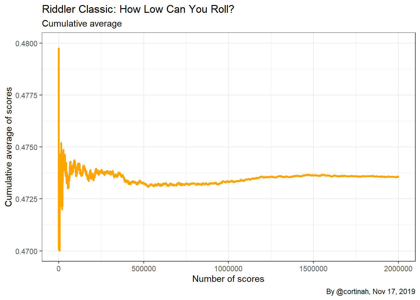
riddler <- mc_table(2000000)

First, I explore the data by simply plotting the scores. It seems to converge somewhere between 0.47 and 0.48.

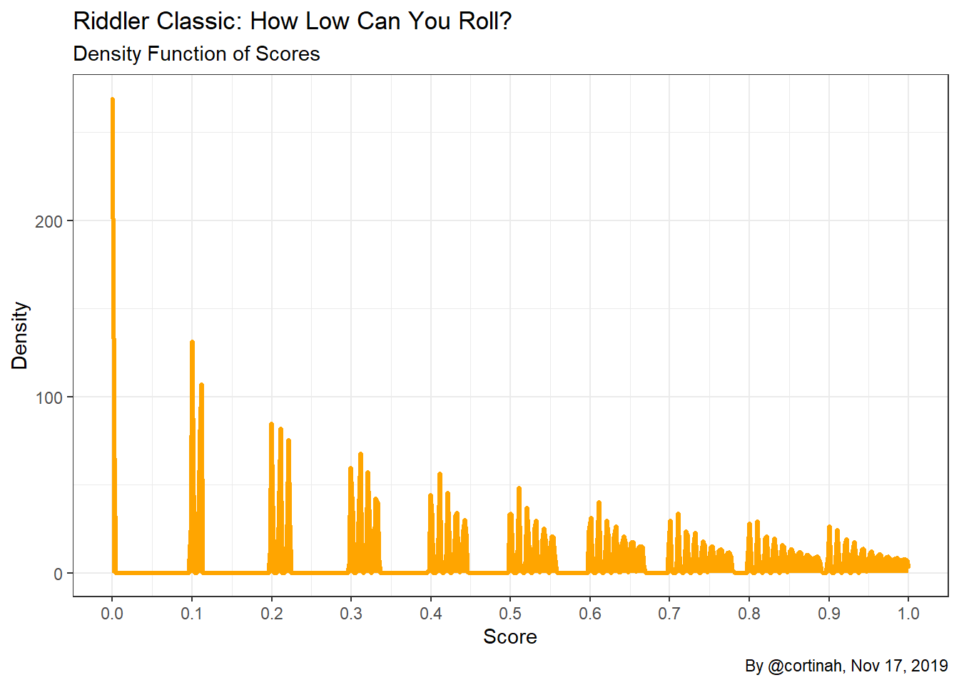
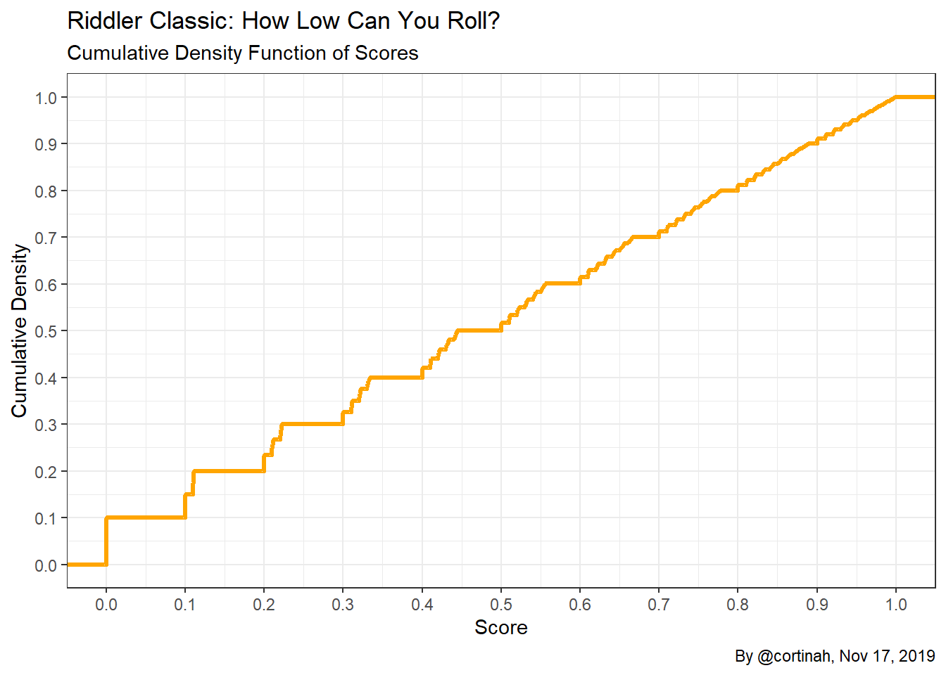
To get a better understanding of the scores the game is generating let’s estimate the probability density function of the process using kernel estimates, as well as the corresponding cumulative density.

Now it is much easier to see how the gaps between scores shrink as we move from 0 to 1. Games that start with a low number such as 0, 1, or 2 remain tightly concentrated near the initial value, while games that start with a higher value such as 7, 8, or 9 can “spread out”. The CDF shows a staircase pattern which becomes less jagged as the score increases due to the samaller gaps in scores.

What’s the final answer?

Below is the calculation of the average score and its standard error. I use the standard deviation divided by the square root of the number of observations to get the standard error.

mean(riddler[,2])

## [1] 0.4736

sd(riddler[,2])/sqrt(2000000)

## [1] 0.0002141

And the answer is… 0.4736 with a standard error of 0.0002141. A 95% confidence interval for the average score is (0.4731, 0.4740). It’s not obvious (at least to me) from the construction of the problem that the average would be near 0.47, or even below 0.5.

Thanks for reading!